This is one in a series of reaction-diffusion tutorials; click here to go to the front page.
Overview
In every cell type, intracellular Ca2+ signaling plays a major role in a diverse set of activities, including process homeostasis and genetic expression. In neurons, Ca2+ wave propagation has been implicated as a major component of intracellular signaling and is complementary to membrane electrical signaling via action potentials. It follows that the cell must contain tightly-controlled intrinsic mechanisms for regulating intracellular Ca2+ content and waves; these include cytosolic buffers, storage in the ER, and sequestration into mitochondria. In this tutorial, we examine how some of these basic mechanisms interact to produce a Ca2+ wave.
Concept
Ca2+ is well-buffered by several cytosolic proteins (e.g. calmodulin, calbindin, etc...), but must still traverse a significant distance within the neuron to reach its targets. This distance is long enough that pure diffusion would pose a temporal problem for cell communication. Instead, the cell uses oscillating Ca2+ waves to harness the power of chemical signaling. These waves can travel up and down the Endoplasmic Reticulum (ER) to effect homeostatic changes. Understanding how these waves are modulated in real time by the cell poses a great difficulty because of complex spatiotemporal patterns and nonuniform distribution of the channels that control Ca2+ flux across the ER. Inositol triphosphate (IP3) receptors IP3Rs), Sarco/endoplasmic reticulum Ca2+-ATPase (SERCA pump), and Ryanoine receptors (RyRs). For simplicity’s sake, we will not deal with RyRs in this tutorial.
Diffusible Ca2+ is released directly from the ER via IP3Rs upon cooperative binding of free Ca2+ and IP3 to the receptor. When IP3 levels are ideal, this results in Ca2+-induced Ca2+ release (CICR), yielding a wave that can travel along the ER. As mentioned above, these waves are implicated in the gene expression and protein upregulation associated with neuronal plasticity by way of their interaction with the neuronal soma. The SERCA pumps within ER are normally responsible for maintaining appropriate intracellular Ca2+ levels. Two models exist for wave propagation: continuous and saltatory. To understand the physical and functional differences between these models, it is ideal to compare them using Reaction-Diffusion (RxD) wtihin the NEURON environment.
The model presented in this tutorial generates Ca2+ waves and is a simplification of the model we used in Neymotin et al., 2015.
Specification
Python is a rich and user-friendly programming language that offers significant options for systems integration. For this reason, we will run the NEURON and RxD modules within the Python interpreter.
Like other RxD problems within NEURON, the first step is to import and load the appropriate libraries into the Python interpreter.
from neuron import h, crxd as rxd
from matplotlib import pyplot
h.load_file('stdrun.hoc')Basic structure
First, we define parameters for the section to be used. Like any imported module within Python, the imported libraries can be accessed by the h and rxd prefixes:
sec = h.Section(name='sec')
sec.L = 101
sec.diam = 1
sec.nseg = 101
The above code defines a section of a neuron with Length = 101 ({\mu}m), diameter = 1 ({\mu}m), and 101 discrete segments. By chunking the neuron into a large number of segments, we increase the resolution of the output at the expense of processing power. For a smaller number of segments, the opposite is true. In larger models, it is useful to represent nseg as a variable – this way, if changes need to be made during any number of simulations, the single variable can be altered and will affect all subsequent iterations of nseg. In this example, we only reference a single section, so there is no need to elaborate.
This tutorial is a work-in-progress and will be expanded with more explanation later. For now, working code and the output follow.
Full code
from neuron import h, crxd as rxd
from matplotlib import pyplot
h.load_file('stdrun.hoc')
sec = h.Section(name='sec')
sec.L = 101
sec.diam = 1
sec.nseg = 101
caDiff = 0.08
ip3Diff = 1.41
cac_init = 1.e-4
ip3_init = 0.1
gip3r = 12040
gserca = 0.3913
gleak = 6.020
kserca = 0.1
kip3 = 0.15
kact = 0.4
ip3rtau = 2000
fc = 0.8
fe = 0.2
average_ca_inside = 0.0017
cyt = rxd.Region(h.allsec(), nrn_region='i', geometry=rxd.FractionalVolume(fc, surface_fraction=1))
er = rxd.Region(h.allsec(), geometry=rxd.FractionalVolume(fe))
cyt_er_membrane = rxd.Region(h.allsec(), geometry=rxd.DistributedBoundary(1))
ca = rxd.Species([cyt, er], d=caDiff, name='ca', charge=2, initial=cac_init, atolscale=1e-6)
ip3 = rxd.Species(cyt, d=ip3Diff, initial=ip3_init)
ip3r_gate_state = rxd.State(cyt_er_membrane, initial=0.8)
h_gate = ip3r_gate_state[cyt_er_membrane]
serca = rxd.MultiCompartmentReaction(ca[cyt], ca[er], gserca / ((kserca / (1000. * ca[cyt])) ** 2 + 1), membrane=cyt_er_membrane, custom_dynamics=True)
leak = rxd.MultiCompartmentReaction(ca[er], ca[cyt], gleak, gleak, membrane=cyt_er_membrane)
minf = ip3[cyt] * 1000. * ca[cyt] / (ip3[cyt] + kip3) / (1000. * ca[cyt] + kact)
k = gip3r * (minf * h_gate) ** 3
ip3r = rxd.MultiCompartmentReaction(ca[er], ca[cyt], k, k, membrane=cyt_er_membrane)
ip3rg = rxd.Rate(h_gate, (1. / (1 + 1000. * ca[cyt] / (0.3)) - h_gate) / ip3rtau)
h.CVode().active(True)
h.finitialize(-65)
cae_init = (average_ca_inside - cac_init * fc) / fe
ca[er].concentration = cae_init
for node in ip3.nodes:
if node.x < 0.2:
node.concentration = 2
# we changed the concentrations, so we must re-init
h.CVode().re_init()
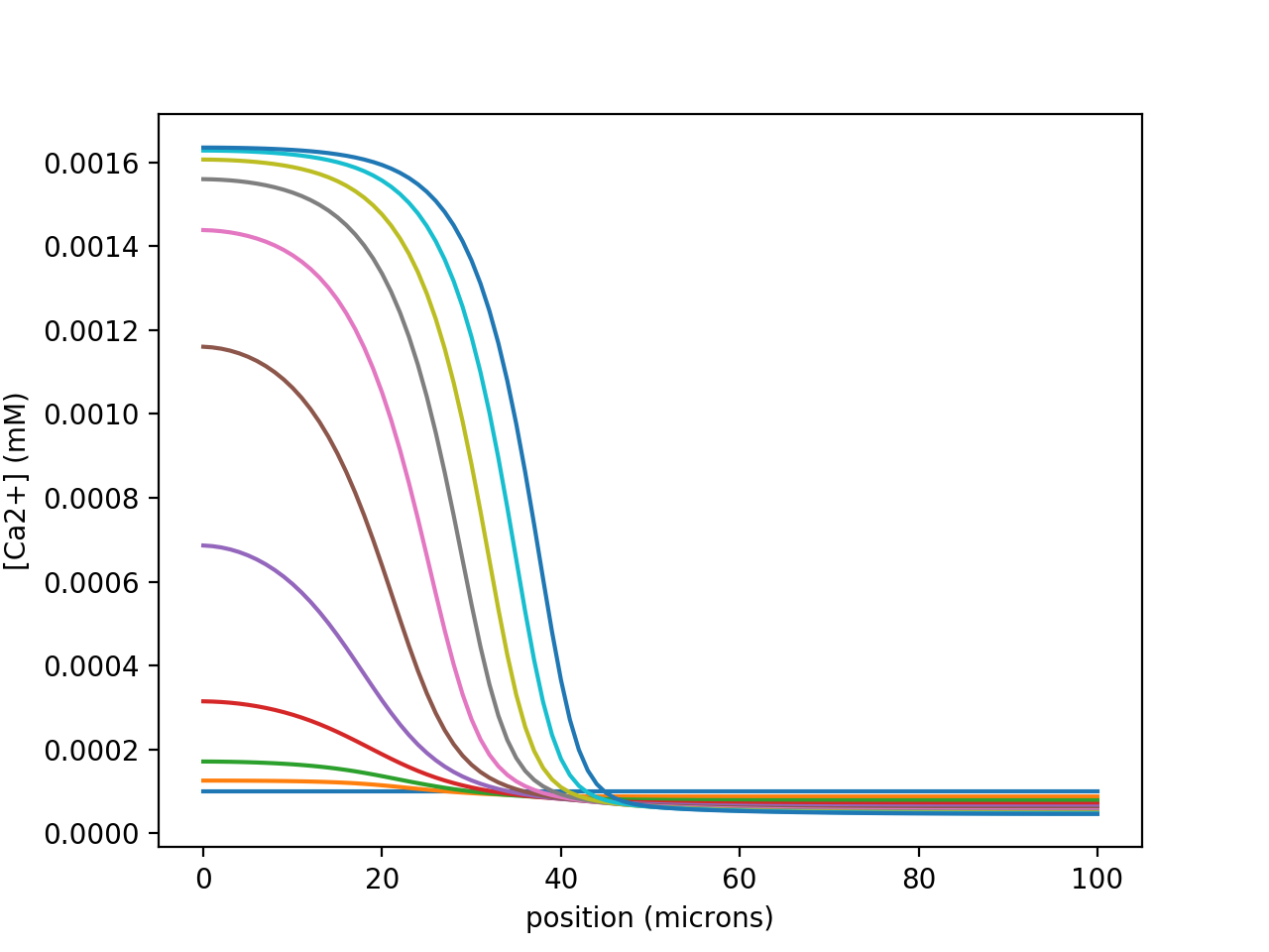
for t in range(0, 501, 50):
h.continuerun(t)
print(t)
pyplot.plot(ca[cyt].concentration)
pyplot.xlabel('position (microns)')
pyplot.ylabel('[Ca2+] (mM)')
pyplot.show()
Output