If you're working on a HOC kernel, I also encourage this...
But:
(1) Consider teaching in Python instead of HOC. That's what we do for the official NEURON courses. The Python programmer's reference is not only the default version, but it's also more up-to-date and has more examples.
(2) As long as you are using Python, then you can embed interactive equivalents of most graphs you might like to do.
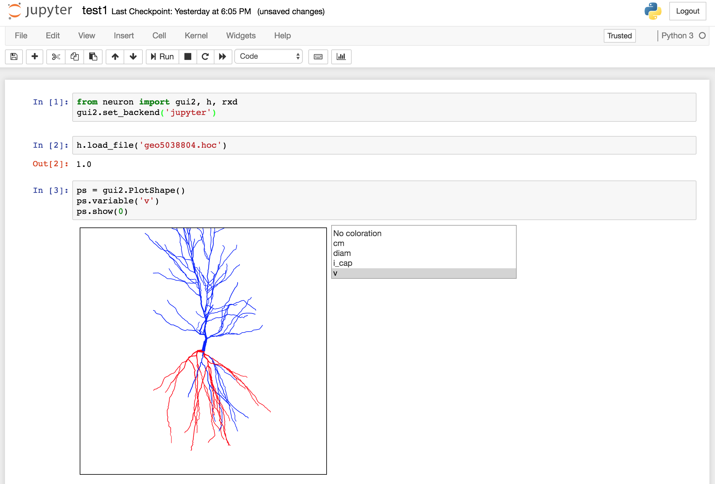
(2a) For example, PlotShape (needs NEURON 7.6.1+; download the latest from
http://neuron.yale.edu):
Code: Select all
from neuron import h, gui2
gui2.set_backend('jupyter')
h.load_file('geo5038804.hoc')  # or whatever morphology you like
ps = gui2.PlotShape()
ps.variable('v')
ps.show(0)
(Obviously, in the figure there is code just off screen that leads to non-uniform membrane potential.)
The PlotShape is interactive (pan, zoom, 3D rotate) and continuously updates (as you'd expect it to) as variables change.
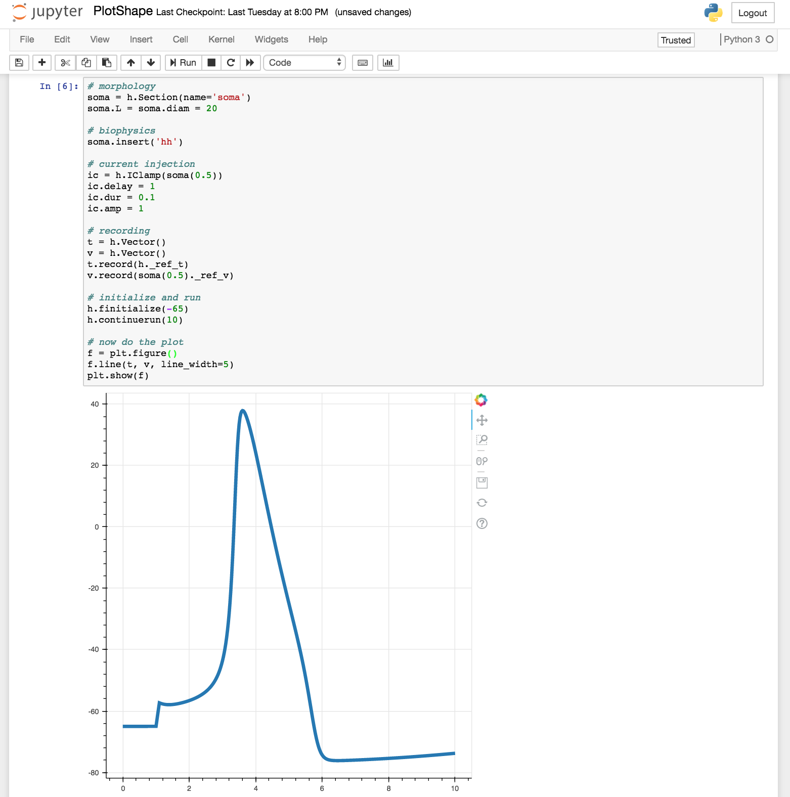
(2b) Plotting time series with bokeh:
Code: Select all
from neuron import h

# using bokeh for graphics
from bokeh.io import output_notebook
import bokeh.plotting as plt
output_notebook()

# standard run library (gives h.continuerun)
h.load_file('stdrun.hoc')

# morphology
soma = h.Section(name='soma')
soma.L = soma.diam = 20

# biophysics
soma.insert('hh')

# current injection
ic = h.IClamp(soma(0.5))
ic.delay = 1
ic.dur = 0.1
ic.amp = 1

# recording
t = h.Vector()
v = h.Vector()
t.record(h._ref_t)
v.record(soma(0.5)._ref_v)

# initialize and run
h.finitialize(-65)
h.continuerun(10)

# now do the plot
f = plt.figure()
f.line(t, v, line_width=5)
plt.show(f)
(2c) Plotting RangeVarPlot (Space Plots) with bokeh:

Code: Select all
from neuron import h

# using bokeh for graphics
from bokeh.io import output_notebook
import bokeh.plotting as plt
output_notebook()

# standard run library (gives h.continuerun)
h.load_file('stdrun.hoc')

# morphology
axon = h.Section(name='axon')
axon.L = 10000
axon.diam = 1
axon.nseg = 101

# biophysics
axon.insert('hh')

# current injection
ic = h.IClamp(axon(0))
ic.delay = 1
ic.dur = 0.1
ic.amp = 1

# setup a plot

# setup rangevarplot
rvp = h.RangeVarPlot('v')
rvp.begin(axon(0))
rvp.end(axon(1))
x = h.Vector()
y = h.Vector()
ys = []

def save_rvp_data():
    rvp.to_vector(y, x)
    ys.append(list(y))

# initialize and run, plotting twice
h.finitialize(-65)
h.continuerun(5)
save_rvp_data()
h.continuerun(10)
save_rvp_data()

# show the plot
f = plt.figure(x_axis_label='position', y_axis_label='v')
f.multi_line([list(x)] * len(ys), ys, color=['black', 'red'], line_width=2)
plt.show(f)
* The main** known issue with the current Jupyter PlotShape is that it won't re-appear when you reopen a saved notebook; you'll have to rerun the code.
** An h.PlotShape can actually do a lot of things; gui2.PlotShape in 7.6.1 does not reproduce all of the API yet, but it does do a lot of it.